Time-Series Analysis
Important Concepts, Handy Techniques, and Some Cautionary Tales
A travel tip…or Zoli as an unintentional travel agent?


This presentation
40 minutes

Superweek
5 days

My last job
5 years

Yehoshua’s intros


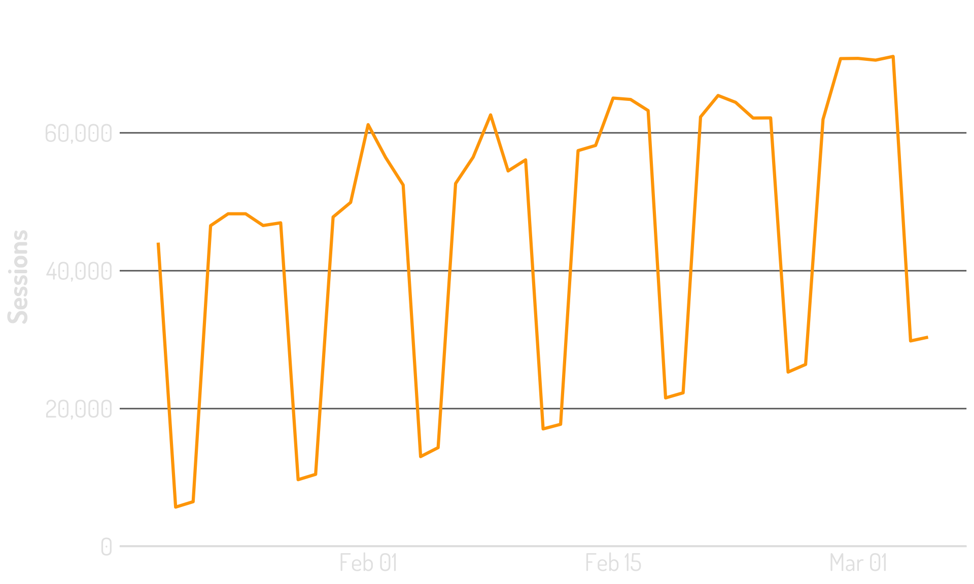
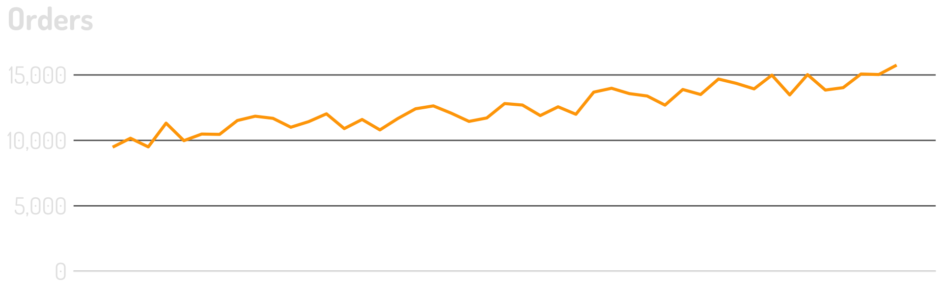
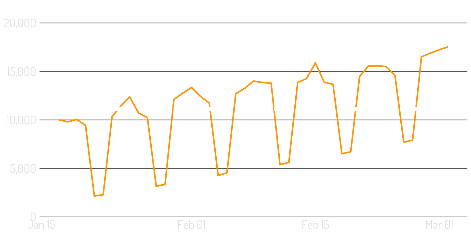
It rarely looks quite like this
It often has a weekly cycle to it

And it may have a trend to it

Let’s think about statistics
Our data exists over time.
So, what is our population?

Is it the past to the present?
Maybe. Maybe not.
Maybe it’s the past, present, and future?
Or…just the future?
But…we can’t sample from the future!
So…what is our sample?
Our sample is a sample timeframe.

This is imperfect.
Because our reality is constant change.
A stationary time series is one whose statistical properties do not depend on the time at which the series is observed. 1
A stationary time series is one whose statistical properties do not depend on the time at which the series is observed. 1
A stationary time series is one whose statistical properties do not depend on the time at which the series is observed. 1
Are these two metrics correlated?
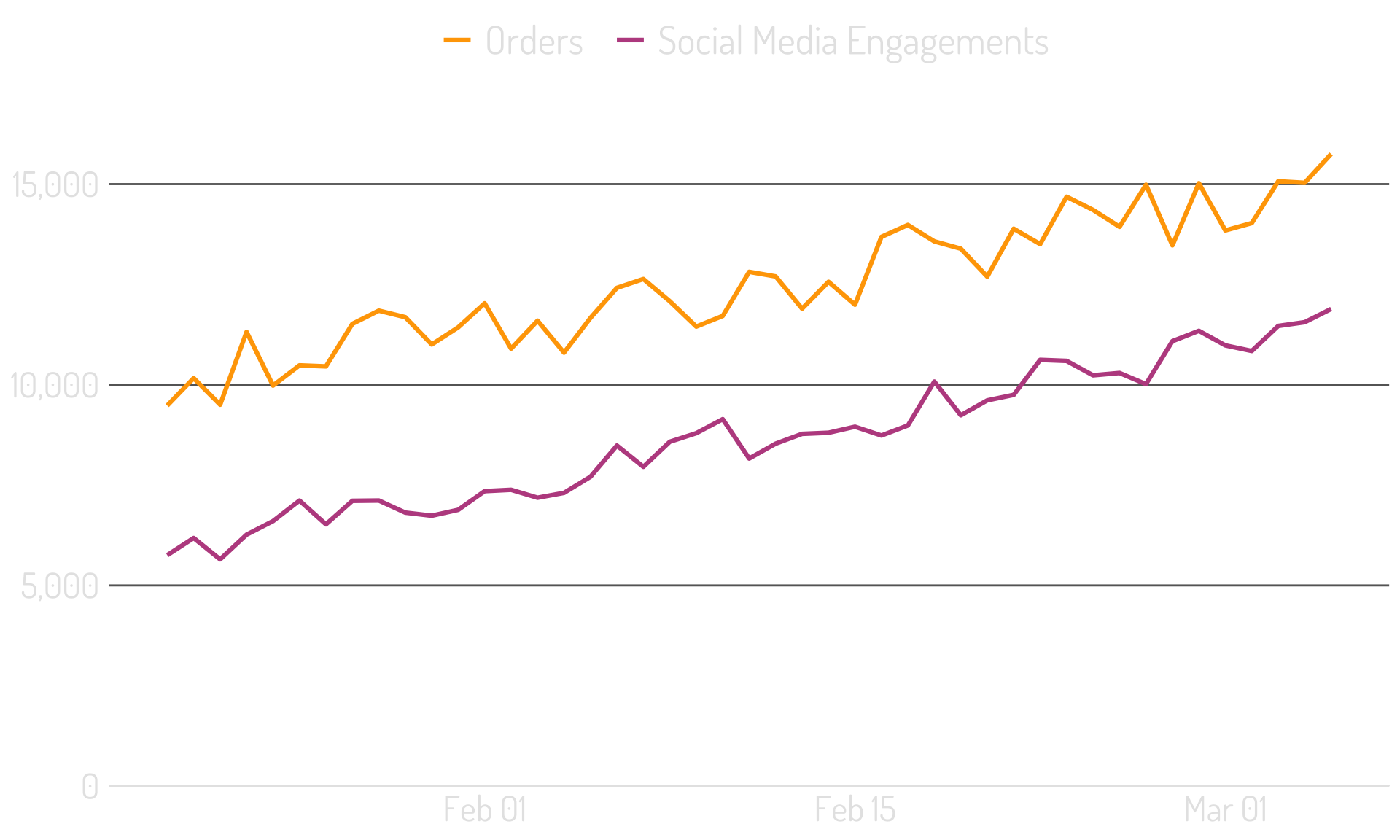
To the scatterplot!
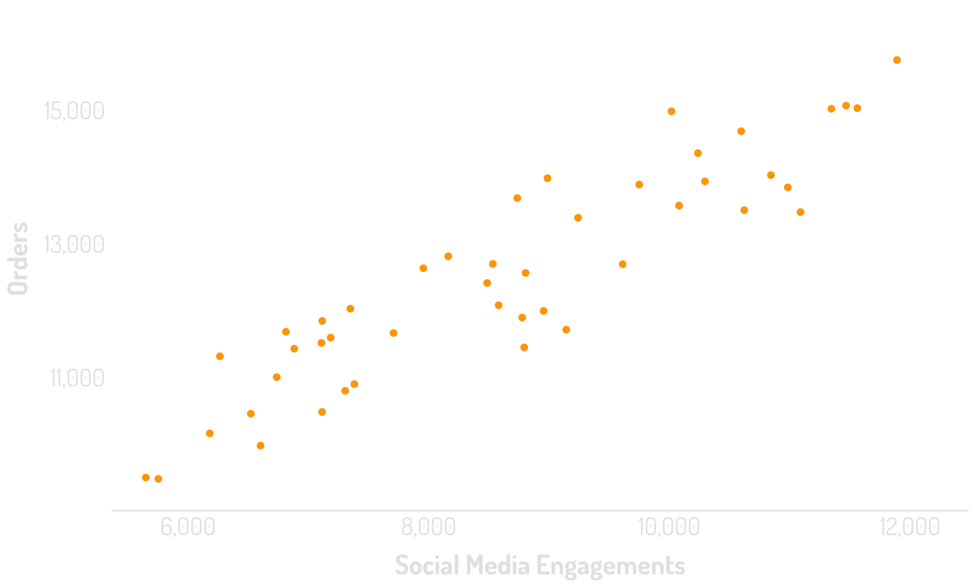
R2 = 0.84


From non-stationary to more stationary
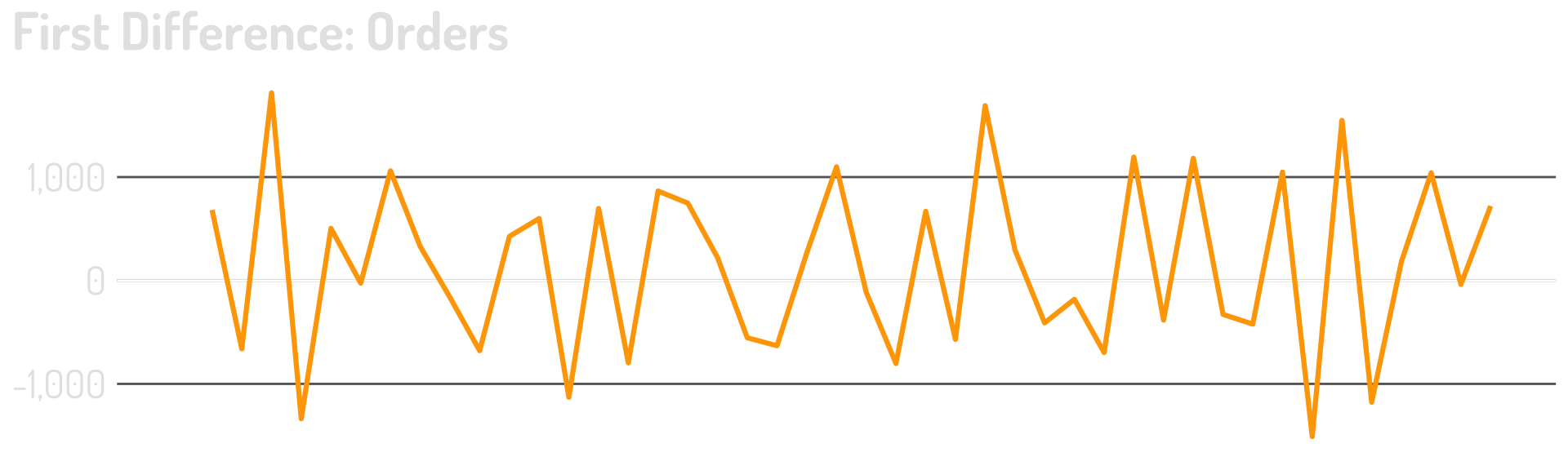
And then check the correlation!
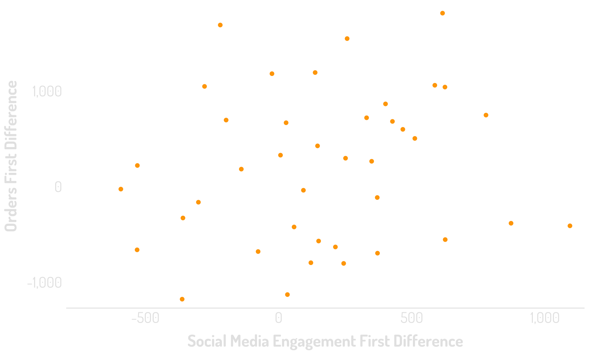
R2 = 0.00
These are both moving with time…but not directly with each other


Let’s shift gears

Decomposition can be amazing
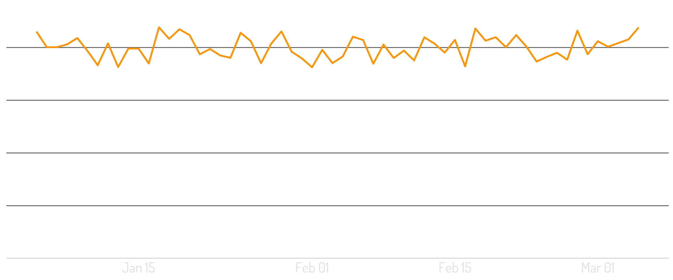
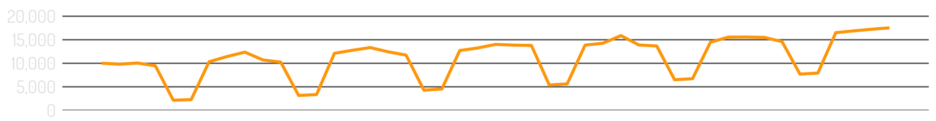
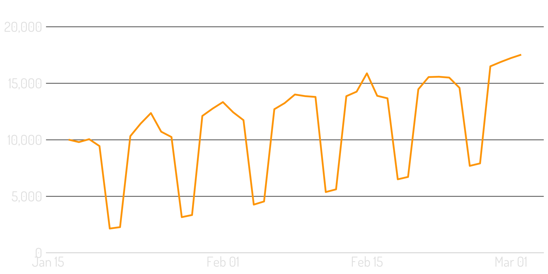
A fairly “clean” series

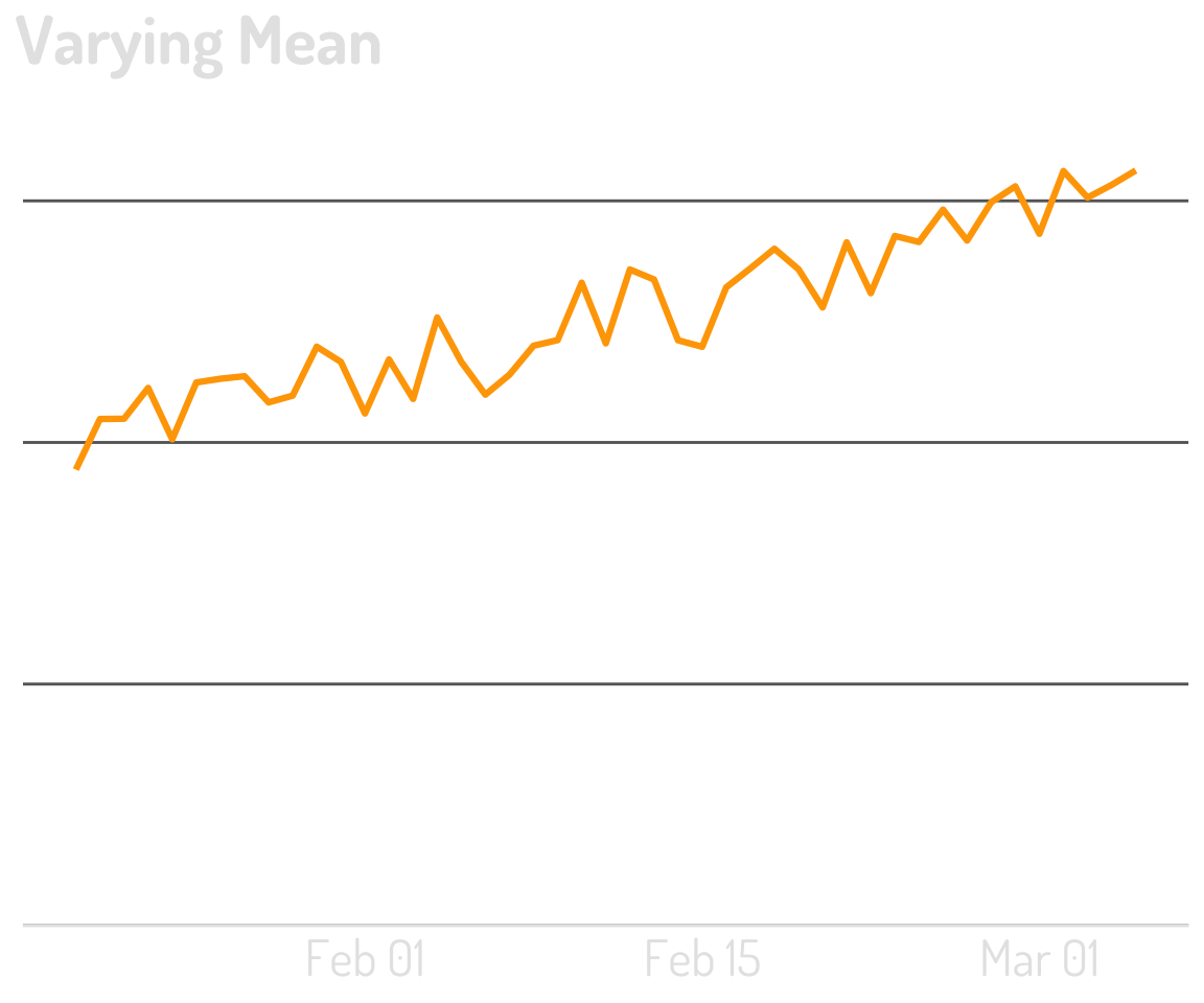
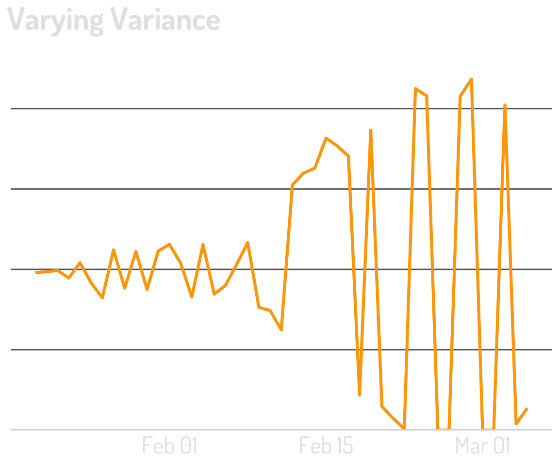
The mean…is pretty meaningless
And so is the variance

It “decomposes” the data into three components

It “decomposes” the data into three components
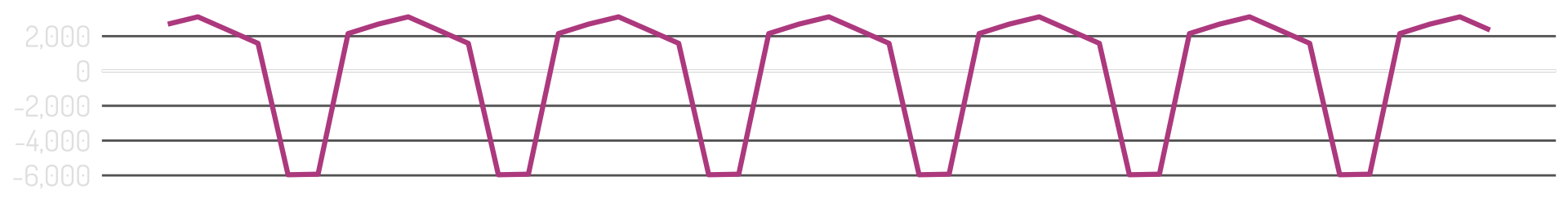
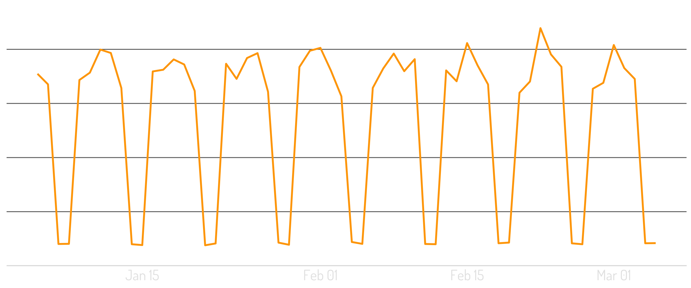
The Seasonal Component
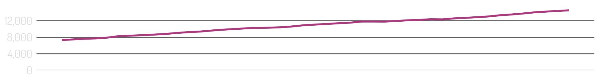
The Trend Component

What’s Left!
“The Mean”
“The Variance”
Back to the overall series

The original mean + variance…embarrassing?
Let’s try again
Seasonality + trend = the “mean”
And the “variance” is just based on “what’s left”

This is powerful!
And now…to Bayesian things!

Specifically, Bayesian Structural Time-Series

Time-series decomposition turned up to 11

Mark Edmondson built a tool using this 7 years ago!
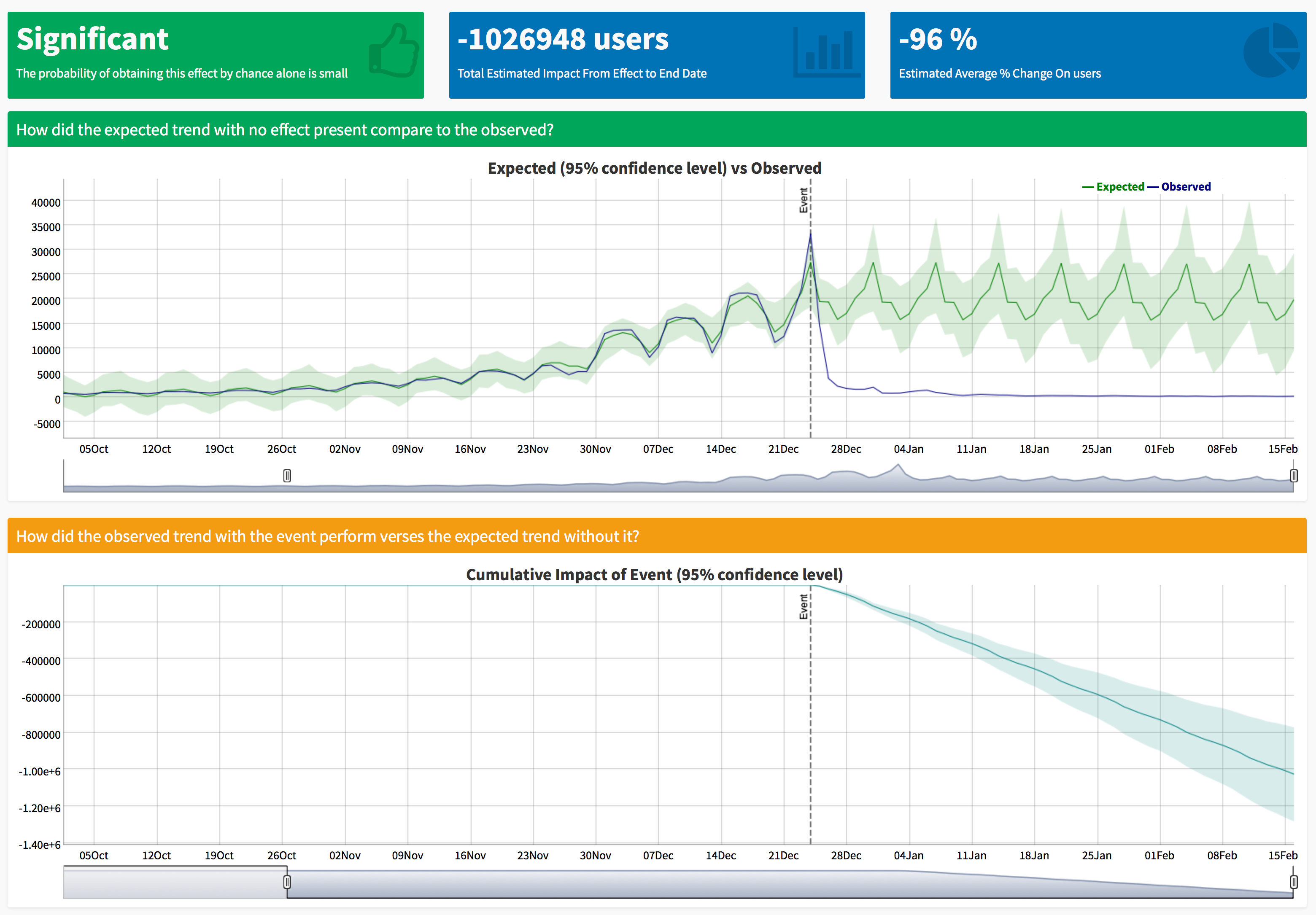
At its core: estimate the impact of an intervention

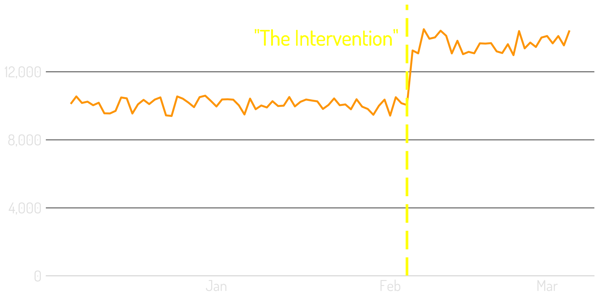
“We didn’t test it, so can we just do a pre-/post- analysis?”

What the marketer expects happened
Typically, the change isn’t that big…
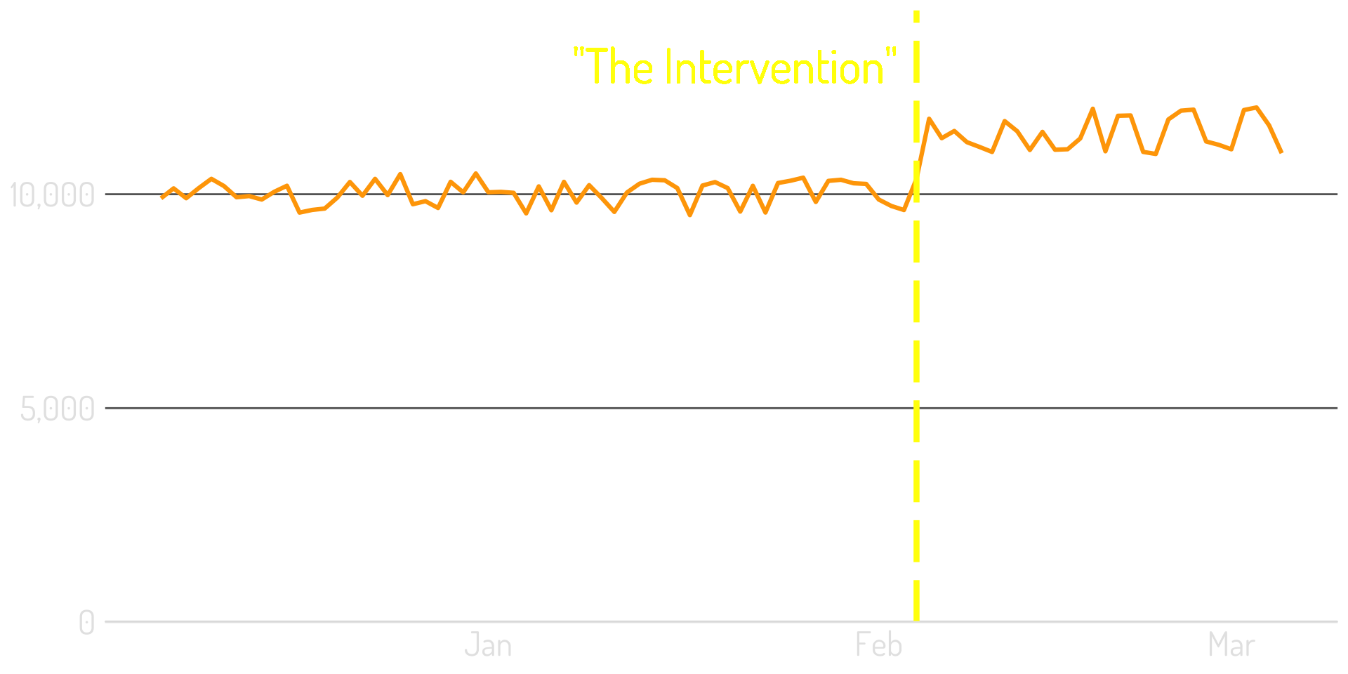
…and the data is a lot noisier…
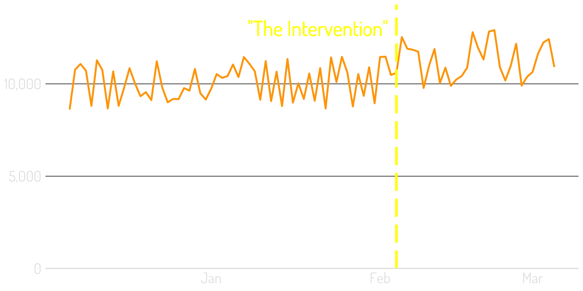
…and may have seasonality!
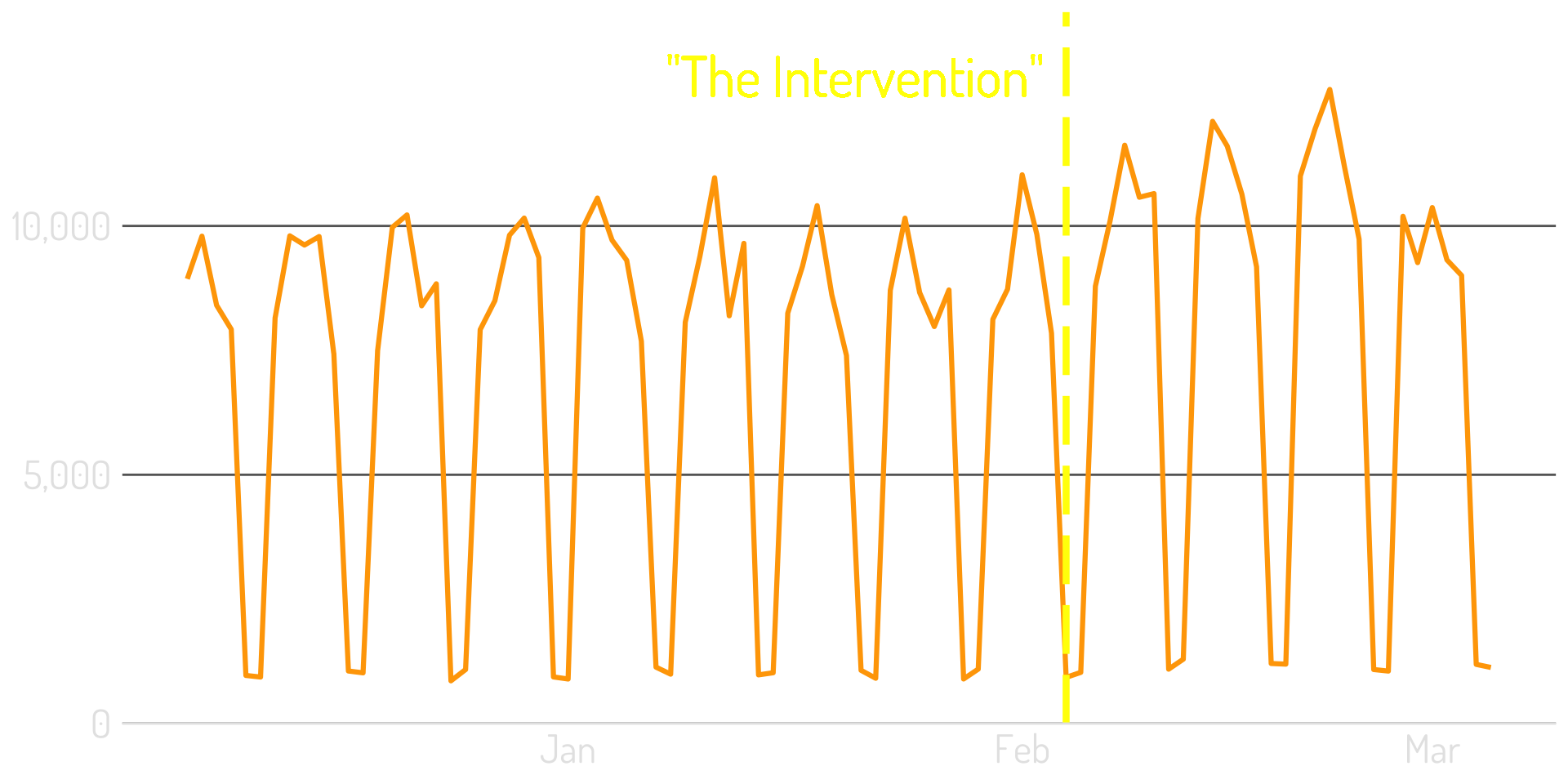
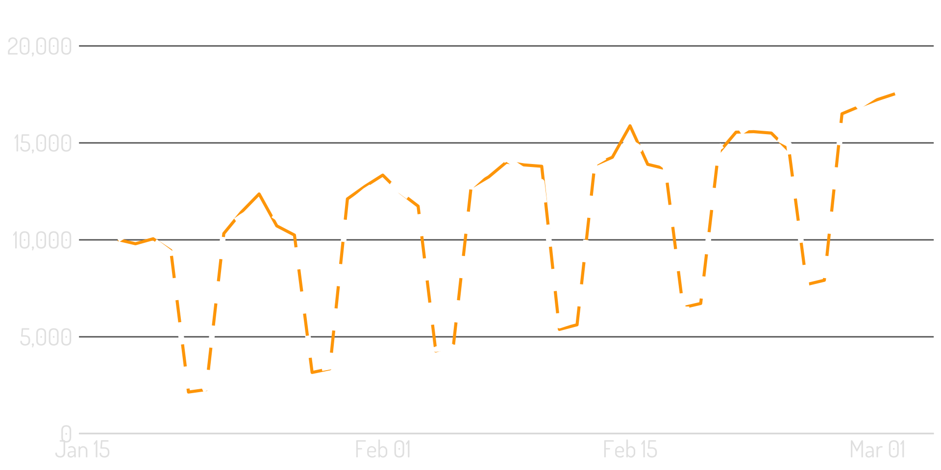
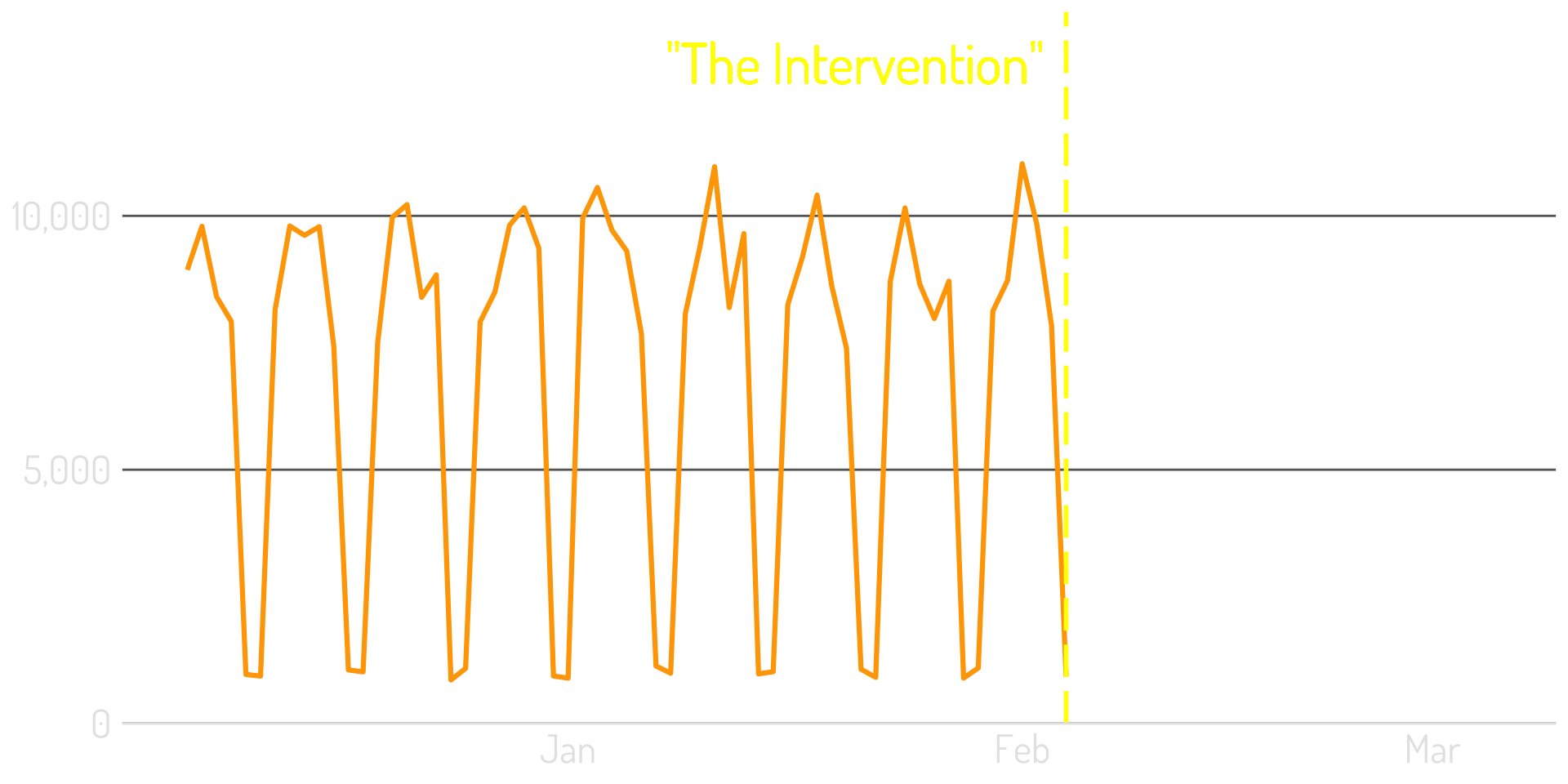
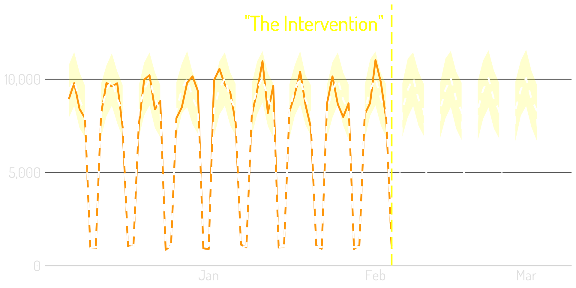
Step 1: Look at the pre-intervention data
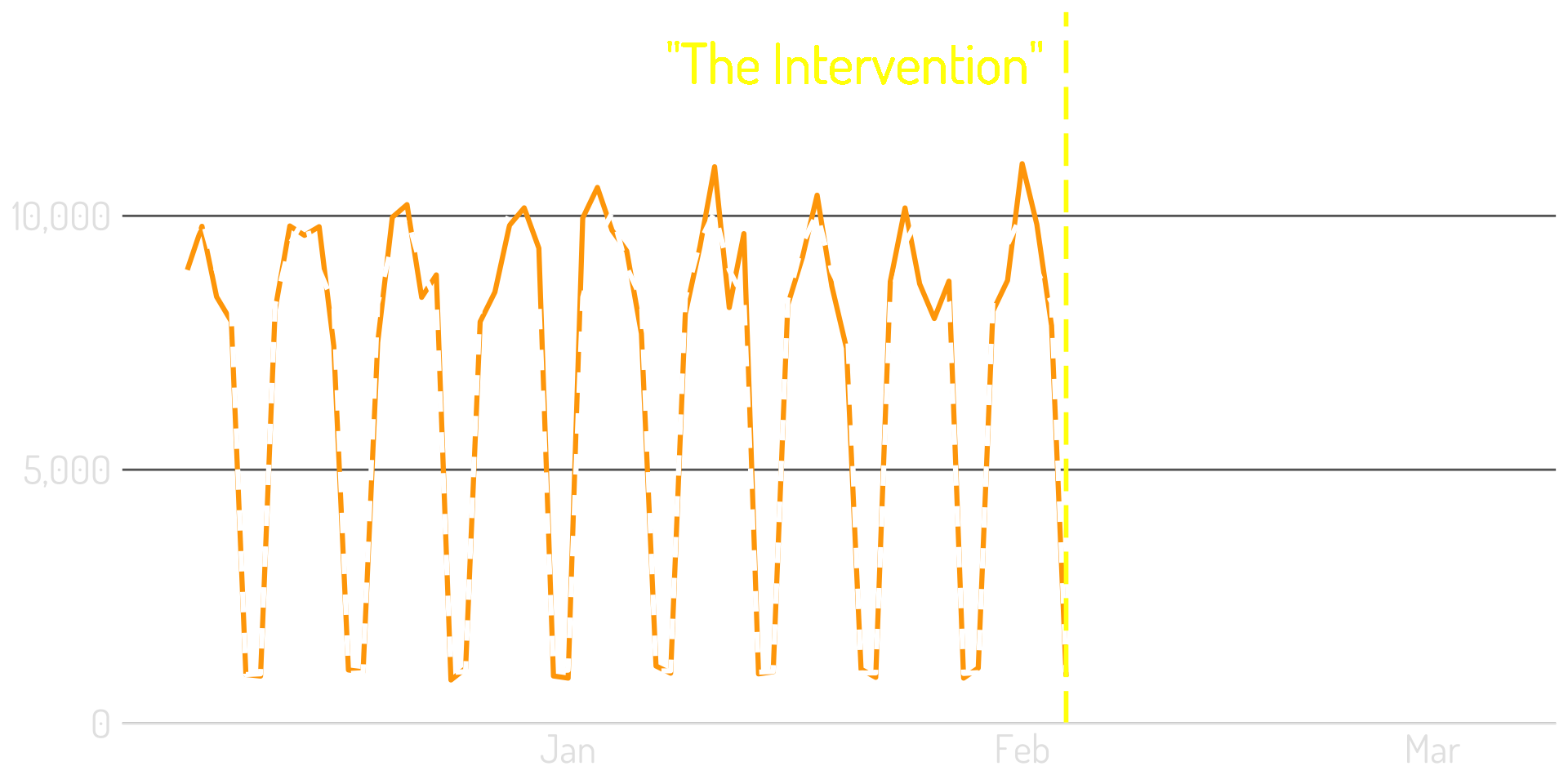
Step 2: Build a best-fit model using this data
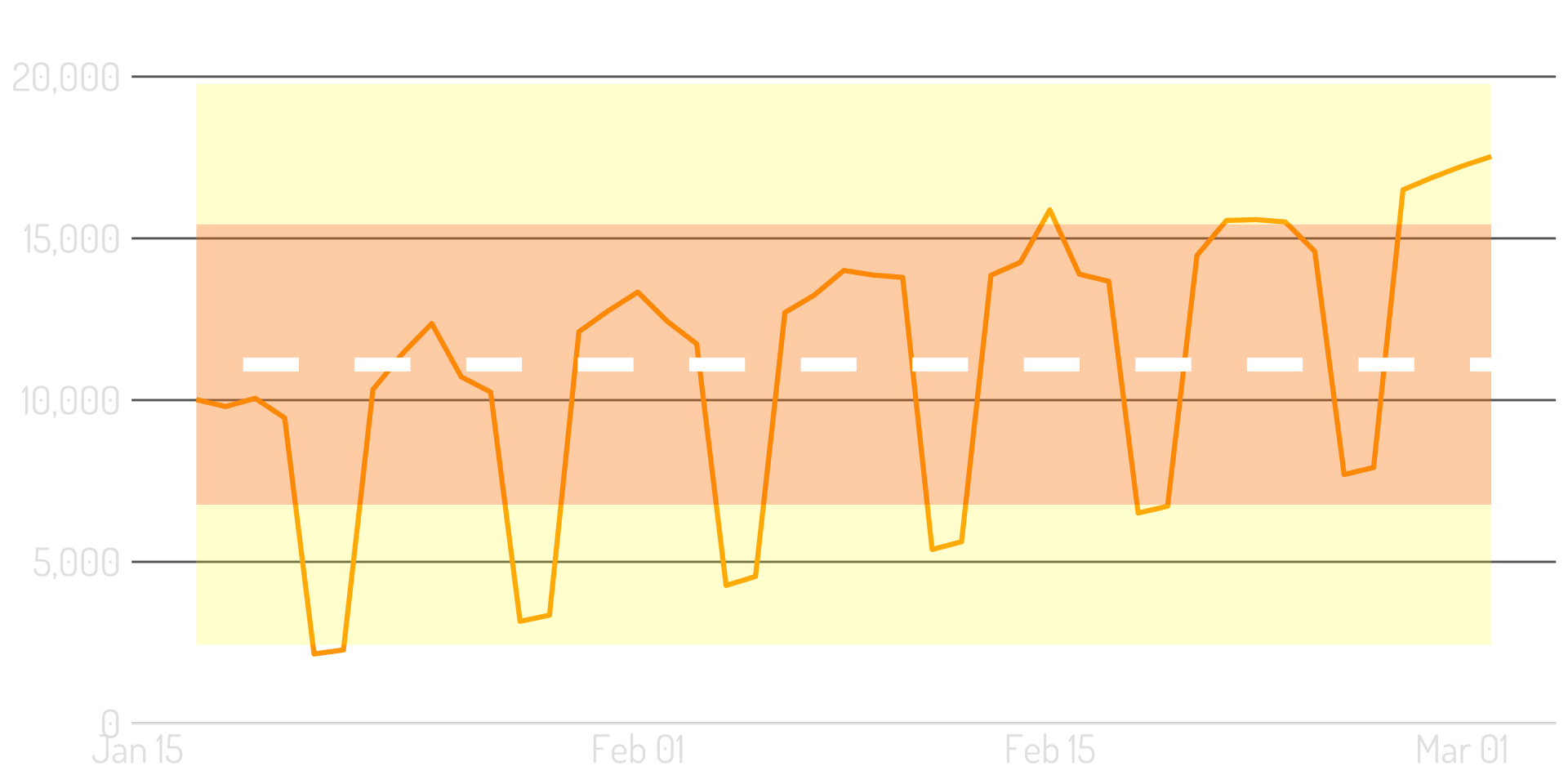
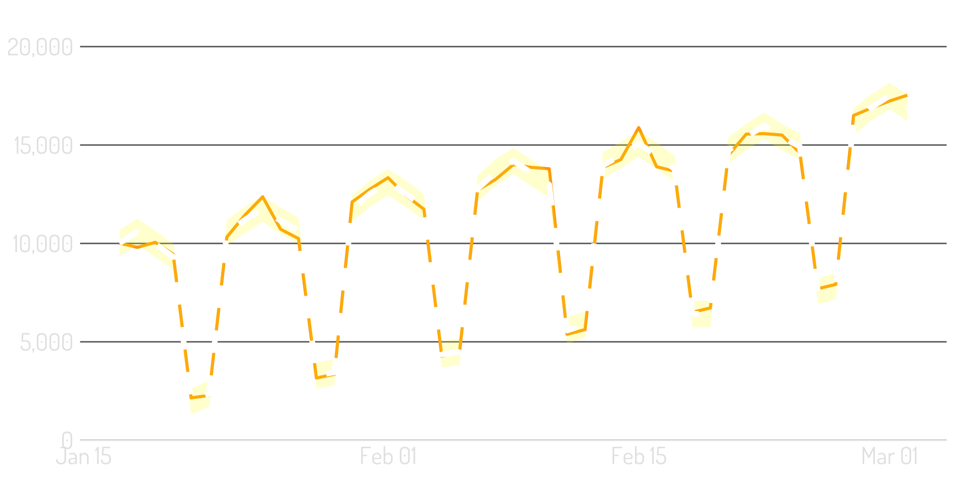
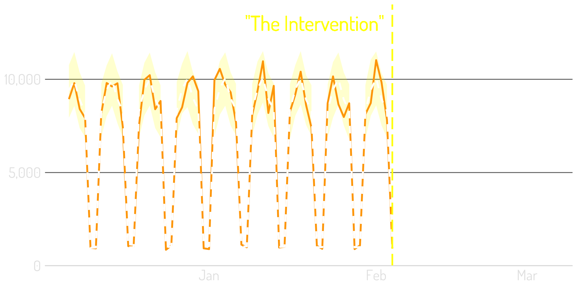
Step 3: That model can quantify its uncertainty
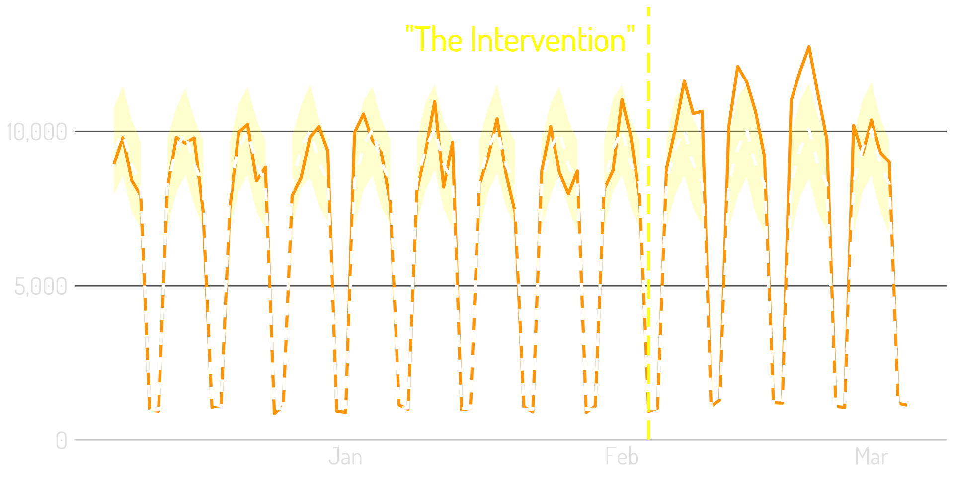
Step 4: Extend the model post-intervention
Step 5: Compare the model to the actual results
Set the modeled prediction as the baseline
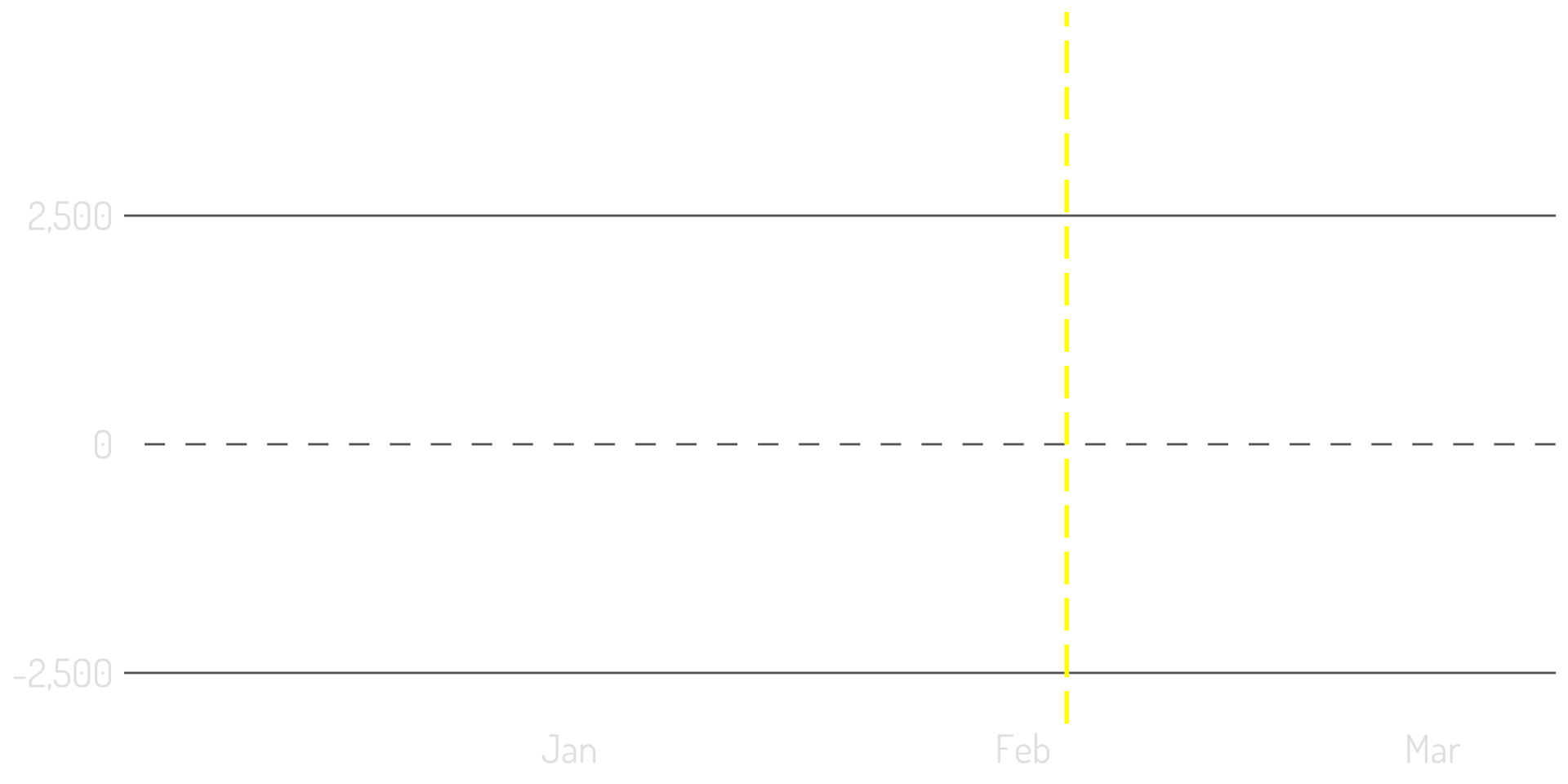
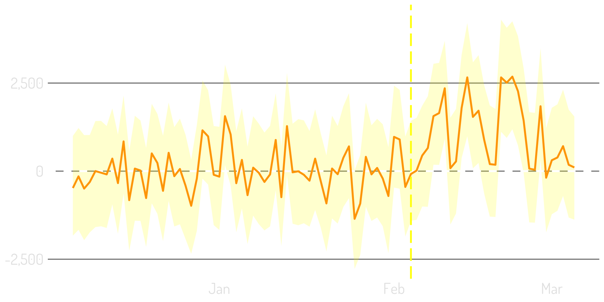
Plot the difference between the model & the actual
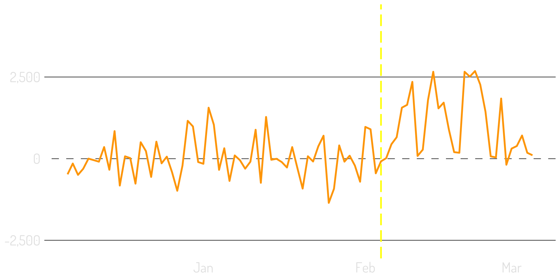
Put the confidence interval around the difference
Their relationship to the metric of interest is stable
They are not themselves affected by the intervention

This is not a silver bullet!

What is “the population?”
Regardless…“the sample” is not ideal
Stationarity: constant mean, constant variance
First differences: don’t jump to correlations
Time-series decomposition
Bayesian structural time-series


Time…is hard.

Thank you!
Presentation: bit.ly/sw-time-series
Podcast: analyticshour.io
LinkedIn:

![]() This presentation was 100% built with R (and Quarto w/ reveal.js)
This presentation was 100% built with R (and Quarto w/ reveal.js)
![]() The images are (almost) 100% DALL-E 2
The images are (almost) 100% DALL-E 2
![]() The background image is from my “daily diversion” on Twitter
The background image is from my “daily diversion” on Twitter